Solutions to tutorial exercises
Solutions to tutorial exercises
import numpy as np
import matplotlib as mpl
import matplotlib.pyplot as plt
from scipy import linalg, interpolate, optimize, special
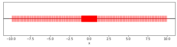
Exercise 02.1:
# 1.

print(2 * 9 * 10 * 3 + 1)

# 2.

print(1.0e-2, 9.9e0)

# 3.

print(1.1e0 - 1.0e0)

# 4.

d_1_vals = [1, 2, 3, 4, 5, 6, 7, 8, 9]
d_2_vals = [0, 1, 2, 3, 4, 5, 6, 7, 8, 9]
E_vals = [0, -1, -2]

fig, ax = plt.subplots(figsize=(10, 2))
ax.axhline(0, color="black")

for E in E_vals:
    for d1 in d_1_vals:
        for d2 in d_2_vals:
            ax.plot(-(d1 + d2 * 0.1) * 10**E, 0.0, color="red", marker="+", markersize=20)
            ax.plot(+(d1 + d2 * 0.1) * 10**E, 0.0, color="red", marker="+", markersize=20)

ax.plot(0.0, 0.0, color="red", marker="+", markersize=20)

ax.set_yticks([])
ax.set_xlabel("x")
ax.set_xlim([-11, 11])
plt.show()
541
0.01 9.9
0.10000000000000009
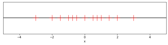
Exercise 02.2:
# 1.

print(2 * 1 * 2 * 3 + 1)

# 2.

print((1.0 * 1.0 + 0.0 * 0.5) * 2.0**(-1), (1.0 * 1.0 + 1.0 * 0.5) * 2.0**1)

# 3.

print((1.0 * 1.0 + 1.0 * 0.5) * 2.0**0 - (1.0 * 1.0 + 0.0 * 0.5) * 2.0**0)

# 4.

d_1_vals = [1]
d_2_vals = [0, 1]
E_vals = [1, 0, -1]

fig, ax = plt.subplots(figsize=(10, 2))
ax.axhline(0, color="black")

for E in E_vals:
    for d1 in d_1_vals:
        for d2 in d_2_vals:
            ax.plot(-(d1 + d2 * 0.5) * 2**E, 0.0, color="red", marker="+", markersize=20)
            ax.plot(+(d1 + d2 * 0.5) * 2**E, 0.0, color="red", marker="+", markersize=20)

ax.plot(0.0, 0.0, color="red", marker="+", markersize=20)

ax.set_yticks([])
ax.set_xlabel("x")
ax.set_xlim([-5, 5])
plt.show()
13
0.5 3.0
0.5
Exercise 02.3:
x = 0.1 + 0.2 - 0.3

for i in range(100):
    x = x + x

print(x)
70368744177664.0
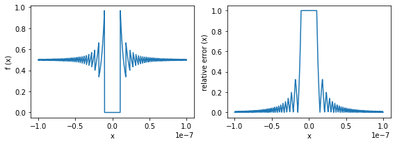
Exercise 02.4:
def function(x):
    return (1.0 - np.cos(x)) / x**2

def relative_error(x):
    return np.abs(0.5 - function(x)) / 0.5

x = np.linspace(-1.0e-7, 1.0e-7, 1000)

fig, ax = plt.subplots(1, 2, figsize=(8, 3))
ax[0].plot(x, function(x))
ax[0].set_xlabel("x")
ax[0].set_ylabel("f (x)")
ax[1].plot(x, relative_error(x))
ax[1].set_xlabel("x")
ax[1].set_ylabel("relative error (x)")
fig.tight_layout()
plt.show()
Exercise 02.5:
array = [0.9**n for n in range(0, 400)]

s_1 = 0.0
for x in array:
    s_1 += x

s_2 = 0.0
for x in array[::-1]:
    s_2 += x

print(s_1, s_2)
9.999999999999993 10.000000000000004
Exercise 02.6:
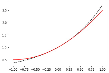
# 1.
x = np.linspace(-1, 1, 100)
def exp_taylor(x):
return 1.0 + x + x**2 / 2.0
fig, ax = plt.subplots()
ax.plot(x, np.exp(x), color="black", linestyle="--")
ax.plot(x, exp_taylor(x), color="red")
plt.show()
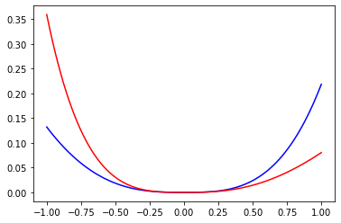
# 2.
def absolute_error(x):
return np.abs(np.exp(x) - exp_taylor(x))
def relative_error(x):
return np.abs(np.exp(x) - exp_taylor(x)) / np.exp(x)
fig, ax = plt.subplots()
ax.plot(x, absolute_error(x), color="blue")
ax.plot(x, relative_error(x), color="red")
plt.show()
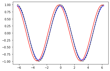
Exercise 02.7:
# 1.
def forward_diff(f, x, h):
return (f(x + h) - f(x)) / h
def central_diff(f, x, h):
return (f(x + h) - f(x - h)) / (2.0 * h)
x = np.linspace(-2.0 * np.pi, 2.0 * np.pi, 1000)
h = 0.5
fig, ax = plt.subplots()
ax.plot(x, forward_diff(np.sin, x, h), color="red")
ax.plot(x, central_diff(np.sin, x, h), color="blue")
ax.plot(x, np.cos(x), color="black", linestyle='--')
plt.show()
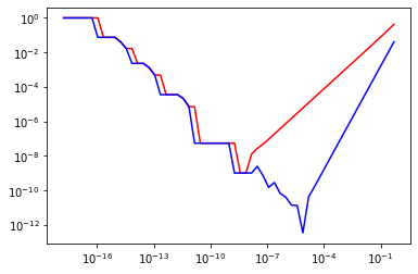
# 2.
def forward_error(f, x, h, exact_value):
return np.abs(forward_diff(f, x, h) - exact_value) / np.abs(exact_value)
def central_error(f, x, h, exact_value):
return np.abs(central_diff(f, x, h) - exact_value) / np.abs(exact_value)
x = 1.0
h = np.array([2.0**(-n) for n in range(1, 60)]);
fig, ax = plt.subplots()
ax.loglog(h, forward_error(np.sin, x, h, np.cos(x)), color="red")
ax.loglog(h, central_error(np.sin, x, h, np.cos(x)), color="blue")
plt.show()
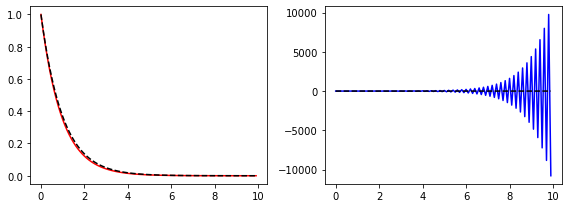
Exercise 02.8:
h = 0.1
x = np.arange(0, 10, h)
y_1 = np.zeros(x.size)
y_2 = np.zeros(x.size)

y_1[0] = 1.0
for i in range(x.size - 1):
    y_1[i+1] = y_1[i] - y_1[i] * h

y_2[0] = 1.0
for i in range(x.size - 1):
    y_2[i+1] = y_2[i-1] - y_2[i] * 2.0 * h

fig, ax = plt.subplots(1, 2, figsize=(8, 3))
ax[0].plot(x, y_1, color="red")
ax[0].plot(x, np.exp(-x), color="black", linestyle="--")
ax[1].plot(x, y_2, color="blue")
ax[1].plot(x, np.exp(-x), color="black", linestyle="--")
fig.tight_layout()
plt.show()
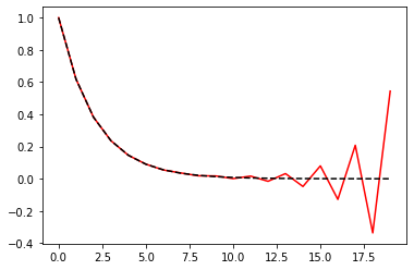
Exercise 02.9:
phi = np.zeros(20, dtype=np.float16)
phi[0] = 1.0
phi[1] = (np.sqrt(5.0) - 1.0) / 2.0
for n in range(1, 19):
    phi[n+1] = phi[n-1] - phi[n]

phi_exact = np.zeros(20, dtype=np.float16)
phi_exact[0] = 1.0
phi_exact[1] = (np.sqrt(5.0) - 1.0) / 2.0
for n in range(1, 19):
    phi_exact[n+1] = phi_exact[n] * phi_exact[1]

fig, ax = plt.subplots()
ax.plot(phi, linestyle="-", color="red")
ax.plot(phi_exact, linestyle="--", color="black")
plt.show()
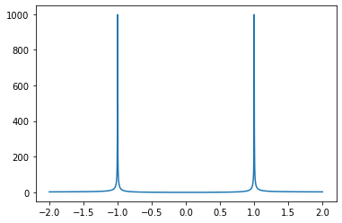
Exercise 02.10:
alpha = np.linspace(-2, 2, 1000)
C_p = 2.0 * alpha**2 / np.abs(1 - alpha**2)

fig, ax = plt.subplots()
ax.plot(alpha, C_p)
plt.show()
Exercise 03.1:
def scalar_product(x, y):
    """
    Calculates scalar product of two vectors.
    Args:
        x (array_like): Vector of size n
        y (array_like): Vector of size n
    Returns:
        numpy.float: Scalar product of x and y
    """
    n = x.size
    z = 0.0
    for i in range(n):
        z = z + x[i] * y[i]
    return z
Exercise 03.2:
def matrix_vector_product(A, x):
    """
    Calculates matrix-vector product.
    Args:
        A (array_like): A m-by-n matrix
        x (array_like): Vector of size n
    Returns:
        numpy.ndarray: Matrix-vector product
    """
    m, n = A.shape
    b = np.zeros(m)
    for i in range(m):
        for j in range(n):
            b[i] = b[i] + A[i, j] * x[j]
    return b
Exercise 03.3:
def matrix_matrix_product(A, B):
    """
    Calculates matrix-matrix product.
    Args:
        A (array_like): A m-by-n matrix
        B (array_like): A n-by-p matrix
    Returns:
        numpy.ndarray: Matrix-matrix product
    """
    m, n = A.shape
    n, p = B.shape
    C = np.zeros((m, p))
    for i in range(m):
        for j in range(p):
            for k in range(n):
                C[i, j] = C[i, j] + A[i, k] * B[k, j]
    return C
Exercise 03.4:
def forward_substitution(A, b):
    """
    Solves a system of linear equations with lower triangular matrix.
    Args:
        A (array_like): A n-by-n lower triangular matrix
        b (array_like): RHS vector of size n
    Returns:
        numpy.ndarray: Vector of solution
    """
    n, n = A.shape
    x = np.zeros(n)
    for i in range(n):
        x[i] = 1.0 / A[i, i] * (b[i] - A[i, :] @ x)
    return x
Exercise 03.5:
def backward_substitution(A, b):
    """
    Solves a system of linear equation with upper triangular matrix.
    Args:
        A (array_like): A n-by-n upper triangular matrix
        b (array_like): RHS vector of size n
    Returns:
        numpy.ndarray: Vector of solution
    """
    n, n = A.shape
    x = np.zeros(n)
    for i in reversed(range(n)):
            x[i] = 1.0 / A[i, i] * (b[i] - A[i, :] @ x)
    return x
Exercise 03.6:
def gaussian_elimination(A):
    """
    Transforms given matrix into an upper triangular form using the Gaussian elimination algorithm.
    Args:
        A (array_like): A n-by-n matrix
    Returns:
        numpy.ndarray: Upper triangular matrix
    """
    n, n = A.shape
    U = np.copy(A)
    for i in range(n):
        for j in range(i + 1, n):
            for k in range(n):
                U[j, k] = U[j, k] - (U[j, i] / U[i, i]) * U[i, k]
    return U
Exercise 03.7:
def gaussian_elimination_with_pivoting(A):
    """
    Transforms given matrix into an upper triangular form using the Gaussian elimination algorithm with pivoting.
    Args:
        A (array_like): A n-by-n matrix
    Returns:
        numpy.ndarray: Upper triangular matrix
    """
    n, n = A.shape
    U = np.copy(A)
    for i in range(n):
        max_row = np.argmax(np.abs(U[i:, i]))
        if (max_row != 0):
            row_i = np.copy(U[i, :])
            U[i, :] = U[i + max_row, :]
            U[i + max_row, :] = row_i
        for j in range(i + 1, n):
            U[j, :] = U[j, :] - (U[j, i] / U[i, i]) * U[i, :]
    return U
Exercise 03.8:
def gaussian_elimination_with_pivoting_vector(A, b):
    """
    Transforms given matrix into an upper triangular form using the Gaussian elimination algorithm with pivoting,
    performs identical operations on RHS vector.
    Args:
        A (array_like): A n-by-n regular matrix
        b (array_like): RHS vector of size n
    Returns:
        numpy.ndarray: Upper triangular matrix
        numpy.ndarray: RHS vector corresponding to upper triangular matrix
    """
    n, n = A.shape
    U = np.zeros((n, n + 1))
    U[:, :-1] = A
    U[:, -1] = b
    for i in range(0, n):
        max_row = np.argmax(np.abs(U[i:, i]))
        if (max_row != 0):
            row_i = np.copy(U[i, :])
            U[i, :] = U[i + max_row, :]
            U[i + max_row, :] = row_i
        for j in range(i + 1, n):
            U[j, :] = U[j, :] - (U[j, i] / U[i, i]) * U[i, :]
    return U[:, :-1], U[:, -1]
Exercise 03.9:
def lu_decomposition(A):
    """
    Factors given matrix as the product of a lower and an upper triangular matrix using LU decomposition.
    Args:
        A (array_like): A n-by-n matrix
    Returns:
        numpy.ndarray: Lower triangular matrix
        numpy.ndarray: Upper triangular matrix
    """
    n, n = A.shape
    L = np.zeros((n, n))
    U = np.zeros((n, n))
    for i in range(n):
        for j in range(i, n):
            U[i, j] = A[i, j] - L[i, :] @ U[:, j]
            L[j, i] = 1.0 / U[i, i] * (A[j, i] - L[j, :] @ U[:, i])
    return L, U
Exercise 03.10:
def thomas_algorithm(A, b):
    """
    Solves system of linear equations with a tridiagonal matrix using Thomas algorithm.
    Args:
        A (array_like): A n-by-n regular matrix
        b (array_like): RHS vector of size n
    Returns:
        numpy.ndarray: Vector of solution
    """
    n, n = A.shape
    p = np.diag(A, 1)
    q = np.diag(A, 0)
    r = np.diag(A, -1)
    p = np.insert(p, n - 1, 0.0)
    r = np.insert(r, 0, 0.0)
    x = np.zeros(n)
    mu  = np.zeros(n)
    rho = np.zeros(n)
    mu[0] = -p[0] / q[0]
    rho[0] = b[0] / q[0]
    for i in range(1, n):
        mu[i] = -p[i] / (r[i] * mu[i - 1] + q[i])
        rho[i] = (b[i] - r[i] * rho[i - 1]) / (r[i] * mu[i - 1] + q[i])
    x[n-1] = rho[n-1]
    for i in reversed(range(n - 1)):
        x[i] = mu[i] * x[i+1] + rho[i]
    return x
Exercise 04.1:
def jacobi_method(A, b, error_tolerance):
    """
    Solves system of linear equations iteratively using Jacobi's algorithm.
    Args:
        A (array_like): A n-by-n diagonally dominant matrix
        b (array_like): RHS vector of size n
        error_tolerance (float): Error tolerance
    Returns:
        numpy.ndarray: Vector of solution
    """
    n, n = A.shape
    x = np.zeros(n)
    x_new = np.zeros(n)
    k = 0
    while linalg.norm(np.dot(A, x) - b) > error_tolerance:
        for i in range(n):
            x_new[i] = (1.0 / A[i, i]) * (b[i]
                - np.dot(A[i, :i], x[:i]) - np.dot(A[i, i+1:], x[i+1:]))
        x = x_new
        k = k + 1
    print(k)
    return x
Exercise 04.2:
def gauss_seidel_method(A, b, error_tolerance):
    """
    Solves system of linear equations iteratively using Gauss-Seidel's algorithm.
    Args:
        A (array_like): A n-by-n diagonally dominant matrix
        b (array_like): RHS vector of size n
        error_tolerance (float): Error tolerance
    Returns:
        numpy.ndarray: Vector of solution
    """
    n, n = A.shape
    x = np.zeros(n)
    k = 0
    while linalg.norm(np.dot(A, x) - b) > error_tolerance:
        for i in range(n):
            x[i] = (1.0 / A[i, i]) * (b[i]
                - np.dot(A[i, :i], x[:i]) - np.dot(A[i, i+1:], x[i+1:]))
        k = k + 1
    print(k)
    return x
Exercise 04.3:
def successive_overrelaxation_method(A, b, omega, error_tolerance):
    """
    Solves system of linear equations iteratively using successive over-relaxation (SOR) method.
    Args:
        A (array_like): A n-by-n matrix
        b (array_like): RHS vector of size n
        omega (float): Relaxation factor
        error_tolerance (float): Error tolerance
    Returns:
        numpy.ndarray: Vector of solution
    """
    n, n = A.shape
    x = np.zeros(n)
    k = 0
    while linalg.norm(np.dot(A, x) - b) > error_tolerance:
        for i in range(n):
            x[i] = (1.0 - omega) * x[i] +  (omega / A[i, i]) * (b[i]
                - np.dot(A[i, :i], x[:i]) - np.dot(A[i, i+1:], x[i+1:]))
        k = k + 1
    print(k)
    return x
Exercise 04.4:
A = np.random.rand(100, 100) + 10 * np.eye(100) # create diagonally dominant matrix to ensure convergence
b = np.random.rand(100)
x = jacobi_method(A, b, 1.0e-15)
x = gauss_seidel_method(A, b, 1.0e-15)
x = successive_overrelaxation_method(A, b, 0.7, 1.0e-15)
103
98
66
Exercise 04.5:
def conjugate_gradient_method(A, b, error_tolerance):
    """
    Solves system of linear equations using conjugate gradient method.
    Args:
        A (array_like): A n-by-n real, symmetric, and positive-definite matrix
        b (array_like): RHS vector of size n
        error_tolerance (float): Error tolerance
    Returns:
        numpy.ndarray: Vector of solution
    """
    n, n = A.shape
    x = np.zeros(n)
    r = b - A @ x
    p = r
    while True:
        alpha = (r.T @ r) / (p.T @ A @ p)
        x = x + alpha * p
        r_new = r - alpha * A @ p
        if linalg.norm(r_new) < error_tolerance:
            break
        beta = (r_new.T @ r_new) / (r.T @ r)
        p = r_new + beta * p
        r = r_new
    return x
Exercise 04.6:
def power_iteration(A, max_it):
    """
    Finds the greatest (in absolute value) eigen value of given matrix and its corresponding eigenvector.
    Args:
        A (array_like): A n-by-n diagonalizable matrix
        max_it (int): Maximum number of iterations
    Returns:
        numpy.ndarray: Eigenvector corresponding to a greatest eigenvalue (in absolute value)
        float: Greatest eigenvalue (in absolute value)
    """
    n, n = A.shape
    e_vec = np.random.rand(n)
    for i in range(max_it):
        e_vec_new = A @ e_vec
        e_vec = e_vec_new / linalg.norm(e_vec_new)
    e_val = linalg.norm(A @ e_vec)
    return e_vec, e_val
Exercise 05.1:
def linear_interpolation(x_p, y_p, x):
    """
    Calculates the linear interpolation.
    Args:
        x_p (array_like): X-coordinates of a set of datapoints
        y_p (array_like): Y-coordinates of a set of datapoints
        x (array_like): An array on which the interpolation is calculated
    Returns:
        numpy.ndarray: The linear interpolation
    """
    sort = np.argsort(x_p)
    x_p = x_p[sort]
    y_p = y_p[sort]
    interp = np.zeros(x.size)
    for i in range(x_p.size - 1):
        interp += (y_p[i] + (y_p[i + 1] - y_p[i]) / (x_p[i + 1] - x_p[i]) *
                   (x - x_p[i])) * (x >= x_p[i]) * (x <= x_p[i + 1])
    return interp
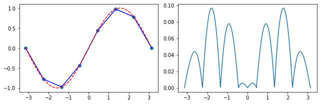
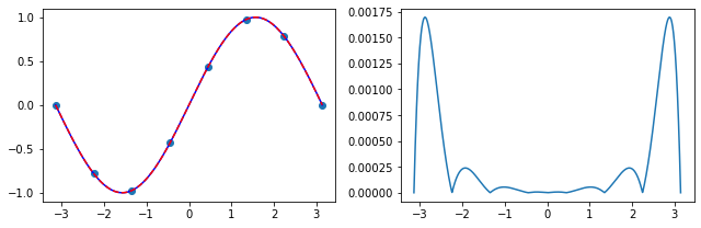
Exercise 05.2:
# create a set of 8 uniformly spaced points from [-pi, pi]
x_p = np.linspace(-np.pi, np.pi, 8)
y_p = np.sin(x_p)

# initialize an array on which the interpolation is evaluated
x = np.linspace(np.min(x_p), np.max(x_p), 1000)

# calculate the piece-wise linear interpolation
f = linear_interpolation(x_p, y_p, x)

# plot the results
fig, ax = plt.subplots(1, 2, figsize=(9, 3))
ax[0].scatter(x_p, y_p)
ax[0].plot(x, f, color="blue")
ax[0].plot(x, np.sin(x), color="red", linestyle="--")
ax[1].plot(x, np.abs(f - np.sin(x)))
fig.tight_layout()
plt.show()
Exercise 05.3:
def lagrange_interpolation(x, y):
    """
    Calculates a Lagrange interpolating polynomial.
    Args:
        x (array_like): X-coordinates of a set of datapoints
        y (array_like): Y-coordinates of a set of datapoints
    Returns:
        numpy.poly1d: The Lagrange interpolating polynomial
    """
    n = x.size
    L = np.poly1d(0)
    for i in range(n):
        F = np.poly1d(1)
        for j in range(n):
            if j != i:
                F *= np.poly1d([1., -x[j]]) / (x[i] - x[j])
        L += y[i] * F
    return L
Exercise 05.4:
# create a set of 8 uniformly spaced points from [-pi, pi]
x_p = np.linspace(-np.pi, np.pi, 8)
y_p = np.sin(x_p)

# initialize an array on which the interpolation is evaluated
x = np.linspace(np.min(x_p), np.max(x_p), 1000)

# calculate the Lagnrange interpolating polynomial
f = lagrange_interpolation(x_p, y_p)

# plot the results
fig, ax = plt.subplots(1, 2, figsize=(9, 3))
ax[0].scatter(x_p, y_p)
ax[0].plot(x, f(x), color="blue")
ax[0].plot(x, np.sin(x), color="red", linestyle="--")
ax[1].plot(x, np.abs(f(x) - np.sin(x)))
fig.tight_layout()
plt.show()
Exercise 05.5:
def neville_algorithm(x, y):
    """
    Calculates a Lagrange interpolating polynomial using Neville's algorithm.
    Args:
        x (array_like): X-coordinates of a set of datapoints
        y (array_like): Y-coordinates of a set of datapoints
    Returns:
        numpy.poly1d: The Lagrange interpolating polynomial
    """
    n = x.size # get the size of data
    L = [[0 for _ in range(n)] for _ in range(n)] # initialize empty list of polynomials
    for i in range(n):
        L[i][i] = np.poly1d(y[i])
    k = 1
    while k < n:
        for i in range(n - k):
            j = i + k
            L[i][j] = (np.poly1d([1., -x[j]]) * L[i][j-1]
                       - np.poly1d([1., -x[i]]) * L[i+1][j]) / (x[i] - x[j])
        k = k + 1
    return L[0][n-1] # return Lagrange polynomial
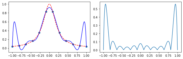
Exercise 05.6:
# define the Runge's function
def runge_function(x):
    return 1.0 / (1.0 + 25.0 * x**2)

# consider a set of points in which the function is evaluated
x_p = np.linspace(-1.0, 1.0, 12)
y_p = runge_function(x_p)

# initialize an array on which the interpolation is evaluated
x = np.linspace(np.min(x_p), np.max(x_p), 1000)

# find Lagrange interpolating polynomial
f = neville_algorithm(x_p, y_p)

# plot results
fig, ax = plt.subplots(1, 2, figsize=(9, 3))
ax[0].scatter(x_p, y_p)
ax[0].plot(x, f(x), color="blue")
ax[0].plot(x, runge_function(x), color="red", linestyle="--")
ax[1].plot(x, np.abs(f(x) - runge_function(x)))
fig.tight_layout()
plt.show()
Exercise 05.7:
def chebyshev_polynomial(n):
    """
    Calculates a Chebyshev polynomial of degree n using recursive formula.
    Args:
        n (int): Degree of the polynomial
    Returns:
        numpy.poly1d: The Chebyshev polynomial of degree n
    """
    T = [0 for i in range(n + 1)]
    for i in range(n + 1):
        if i == 0:
            T[i] = np.poly1d(1)
        elif i == 1:
            T[i] = np.poly1d([1, 0])
        else:
            T[i] = 2.0 * np.poly1d([1, 0]) * T[i-1] - T[i-2]
    return T[n]
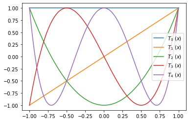
Exercise 05.8:
x = np.linspace(-1.0, 1.0, 1000)

# plot Chebyshev polynomials
fig, ax = plt.subplots()
for i in range(5):
    T = chebyshev_polynomial(i)
    ax.plot(x, T(x), label=r"$ T_{} \ (x) $".format(i))
ax.legend()
plt.show()
Exercise 05.9:
def chebyshev_roots(n):
    """
    Calculates roots of a Chebyshev polynomial of degree n.
    Args:
        n (int): Degree of the polynomial
    Returns:
        numpy.ndarray: Roots of a Chebyshev polynomial of degree n
    """
    roots = np.zeros(n)
    for k in range(n):
        roots[k] = -np.cos(np.pi * (k + 0.5) / n)
    return roots
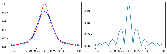
Exercise 05.10:
# define the Runge's function
def runge_function(x):
    return 1.0 / (1.0 + 25.0 * x**2)

# evaluate the Runge's function at roots of the 12-th degree Chebyshev polynomial
x_p = chebyshev_roots(12)
y_p = runge_function(x_p)

# initialize an array on which the interpolation is calculated
x = np.linspace(-1.0, 1.0, 1000)

# calculate the Lagrange interpolating polynomial
f = neville_algorithm(x_p, y_p)

# plot the results
fig, ax = plt.subplots(1, 2, figsize=(9, 3))
ax[0].scatter(x_p, y_p)
ax[0].plot(x, f(x), color="blue")
ax[0].plot(x, runge_function(x), color="red", linestyle="--")
ax[1].plot(x, np.abs(f(x) - runge_function(x)))
fig.tight_layout()
plt.show()
Exercise 05.11:
def polynomial_least_squares(x, y, n):
    """
    Calculates the n-th degree polynomial least squares approximation.
    Args:
        x (array_like): X-coordinates of a set of datapoints
        y (array_like): Y-coordinates of a set of datapoints
        n (int): degree of the approximating polynomial
    Returns:
        numpy.poly1d: The n-th degree polynomial least squares approximation
    """
    A = np.zeros((n + 1, n + 1))
    b = np.zeros(n + 1)
    for i in range(n + 1):
        b[i] = np.sum(y * x**i)
        for j in range(n + 1):
            A[i, j] = np.sum(x**(i + j))
    beta = linalg.solve(A, b)
    return np.poly1d(beta[::-1])
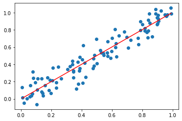
Exercise 05.12:
# consider data with Gaussian noise
x_p = np.random.rand(100)
y_p = x_p + 0.1 * np.random.normal(size=100)

# initialize an array on which the interpolation is evaluated
x = np.linspace(np.min(x_p), np.max(x_p), 100)

# find least squares interpolation
f = polynomial_least_squares(x_p, y_p, 1)

# plot results
fig, ax = plt.subplots()
ax.scatter(x_p, y_p) # plot the discrete data
ax.plot(x, f(x), color="red") # plot least squares interpolation
[<matplotlib.lines.Line2D at 0x2a030e73100>]
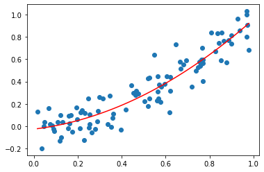
Exercise 05.13:
# consider data with Gaussian noise
x_p = np.random.rand(100)
y_p = x_p**2 + 0.1 * np.random.normal(size=100)

# initialize an array on which the interpolation is evaluated
x = np.linspace(np.min(x_p), np.max(x_p), 100)

# calculate the quadratic least squares interpolation
f = polynomial_least_squares(x_p, y_p, 2)

# plot the result
fig, ax = plt.subplots()
ax.scatter(x_p, y_p) # plot the discrete data
ax.plot(x, f(x), color="red") # plot least squares interpolation
[<matplotlib.lines.Line2D at 0x2a030e377c0>]
Exercise 06.1:
def bubble_sort(array):
    """
    Sorts the input data using bubble sort algorithm.
    Args:
        array (array_like): input data
    Returns:
        numpy.ndarray: sorted data
    """
    tmp = np.copy(array)
    for i in range(tmp.size):
        for j in range(tmp.size - i - 1):
            if tmp[j] > tmp[j + 1]:
                tmp[j], tmp[j + 1] = tmp[j + 1], tmp[j]
    return tmp
Exercise 06.2:
def selection_sort(array):
    """
    Sorts the input data using selection sort algorithm.
    Args:
        array (array_like): input data
    Returns:
        numpy.ndarray: sorted data
    """
    tmp = np.copy(array)
    for i in range(tmp.size):
        index_of_min = i
        for j in range(i, tmp.size):
            if tmp[j] < tmp[index_of_min]:
                index_of_min = j
        #index_of_min = i + np.argmin(tmp[i:])
        if index_of_min != i:
            tmp[i], tmp[index_of_min] = tmp[index_of_min], tmp[i]
    return tmp
Exercise 06.3:
def insertion_sort(array):
    """
    Sorts the input data using inserion sort algorithm.
    Args:
        array (array_like): input data
    Returns:
        numpy.ndarray: sorted data
    """
    tmp = np.copy(array)
    for i in range(1, tmp.size):
        j = i
        val = tmp[i]
        while j > 0 and tmp[j - 1] > val:
            tmp[j] = tmp[j - 1]
            j = j - 1
        tmp[j] = val
    return tmp
Exercise 06.4:
def shell_sort(array):
    """
    Sorts the input data using shell sort algorithm.
    Args:
        array (array_like): input data
    Returns:
        numpy.ndarray: sorted data
    """
    tmp = np.copy(array)
    gap = int(tmp.size / 2)
    while gap > 0:
        for i in range(gap, tmp.size):
            val = tmp[i]
            j = i
            while j >= gap and tmp[j - gap] > val:
                tmp[j] = tmp[j - gap]
                j = j - gap
            tmp[j] = val
        gap = int(gap / 2)
    return tmp
Exercise 06.5:
def quick_sort(array):
    """
    Sorts the input data using quicksort algorithm.
    Args:
        array (array_like): input data
    Returns:
        numpy.ndarray: sorted data
    """
    less = np.array([])
    equal = np.array([])
    greater = np.array([])
    if array.size > 1:
        pivot = array[0]
        for x in array:
            if x < pivot: less = np.append(less, x)
            if x == pivot: equal = np.append(equal, x)
            if x > pivot: greater = np.append(greater, x)
        return np.concatenate((quick_sort(less), equal, quick_sort(greater)))
    else:
        return array
Exercise 06.6:
def heap_sort(array):
    """
    Sorts the input data using heap sort algorithm.
    Args:
        array (array_like): input data
    Returns:
        numpy.ndarray: sorted data
    """
    def heapify(array, size, parent_index):
        index_of_largest = parent_index
        left_child_index = 2 * parent_index + 1
        right_child_index = 2 * parent_index + 2
        if left_child_index < size and array[left_child_index] > array[index_of_largest]:
            index_of_largest = left_child_index
        if right_child_index < size and array[right_child_index] > array[index_of_largest]:
            index_of_largest = right_child_index
        if index_of_largest != parent_index:
            array[index_of_largest], array[parent_index] = array[parent_index], array[index_of_largest]
            heapify(array, size, index_of_largest)
    tmp = np.copy(array)
    for i in reversed(range(int(tmp.size / 2))):
        heapify(tmp, tmp.size, i)
    for i in reversed(range(1, tmp.size)):
        tmp[i], tmp[0] = tmp[0], tmp[i]
        heapify(tmp, i, 0)
    return tmp
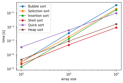
Exercise 06.7:
sizes = [10**i for i in range(1, 4)]

bubblesort_times = []
selectionsort_times = []
insertionsort_times = []
shellsort_times = []
quicksort_times = []
heapsort_times = []
for i in sizes:
    random_array = np.random.rand(i)
    print("bubble sort:")
    time = %timeit -o bubble_sort(random_array)
    bubblesort_times.append(time.average)
    print("selection sort:")
    time = %timeit -o selection_sort(random_array)
    selectionsort_times.append(time.average)
    print("insertion sort:")
    time = %timeit -o insertion_sort(random_array)
    insertionsort_times.append(time.average)
    print("shell sort:")
    time = %timeit -o shell_sort(random_array)
    shellsort_times.append(time.average)
    print("quicksort:")
    time = %timeit -o quick_sort(random_array)
    quicksort_times.append(time.average)
    print("heapsort:")
    time = %timeit -o heap_sort(random_array)
    heapsort_times.append(time.average)

fig, ax = plt.subplots()
ax.loglog(sizes, bubblesort_times, label="Bubble sort", marker="o")
ax.loglog(sizes, selectionsort_times, label="Selection sort", marker="o")
ax.loglog(sizes, insertionsort_times, label="Insertion sort", marker="o")
ax.loglog(sizes, shellsort_times, label="Shell sort", marker="o")
ax.loglog(sizes, quicksort_times, label="Quick sort", marker="o")
ax.loglog(sizes, heapsort_times, label="Heap sort", marker="o")
ax.set_xlabel('array size')
ax.set_ylabel('time [s]')
ax.legend()
plt.show()
bubble sort:
29 µs ± 776 ns per loop (mean ± std. dev. of 7 runs, 10000 loops each)
selection sort:
29.2 µs ± 998 ns per loop (mean ± std. dev. of 7 runs, 10000 loops each)
insertion sort:
13.2 µs ± 374 ns per loop (mean ± std. dev. of 7 runs, 100000 loops each)
shell sort:
20.7 µs ± 1.8 µs per loop (mean ± std. dev. of 7 runs, 100000 loops each)
quicksort:
342 µs ± 6.12 µs per loop (mean ± std. dev. of 7 runs, 1000 loops each)
heapsort:
44 µs ± 1.23 µs per loop (mean ± std. dev. of 7 runs, 10000 loops each)
bubble sort:
3.43 ms ± 112 µs per loop (mean ± std. dev. of 7 runs, 100 loops each)
selection sort:
1.89 ms ± 45.3 µs per loop (mean ± std. dev. of 7 runs, 1000 loops each)
insertion sort:
1.36 ms ± 40.8 µs per loop (mean ± std. dev. of 7 runs, 1000 loops each)
shell sort:
493 µs ± 10 µs per loop (mean ± std. dev. of 7 runs, 1000 loops each)
quicksort:
5.54 ms ± 60.9 µs per loop (mean ± std. dev. of 7 runs, 100 loops each)
heapsort:
901 µs ± 18.9 µs per loop (mean ± std. dev. of 7 runs, 1000 loops each)
bubble sort:
339 ms ± 11.2 ms per loop (mean ± std. dev. of 7 runs, 1 loop each)
selection sort:
183 ms ± 2.5 ms per loop (mean ± std. dev. of 7 runs, 10 loops each)
insertion sort:
155 ms ± 6.42 ms per loop (mean ± std. dev. of 7 runs, 10 loops each)
shell sort:
8.59 ms ± 439 µs per loop (mean ± std. dev. of 7 runs, 100 loops each)
quicksort:
92.8 ms ± 3.9 ms per loop (mean ± std. dev. of 7 runs, 10 loops each)
heapsort:
15 ms ± 700 µs per loop (mean ± std. dev. of 7 runs, 100 loops each)
Exercise 07.1:
def bisection(f, a, b, error_tolerance=1.0e-15, max_iterations=500):
    """
    Finds the root of a continuous function using bisection method.
    Args:
        f (function): Continuous function defined on an interval [a, b], where f(a) and f(b) have opposite signs
        a (float): Leftmost point of the interval
        b (float): Rightmost point of the interval
        error_tolerance (float): Error tolerance
        max_iterations (int): Maximum number of iterations
    Returns:
        float: The root of function f
    Raises:
        RuntimeError: Raises an exception when the root is not found
    """
    k = 0
    while k < max_iterations:
        c = (a + b) / 2.0
        if f(a) * f(c) > 0:
            a = c
        else:
            b = c
        k = k + 1
        if np.abs(b - a) < error_tolerance:
            print("root found within tolerance", error_tolerance, "using", k, "iterations")
            return (a + b) / 2.0
    raise RuntimeError("no root found within tolerance", error_tolerance, "using", max_iterations, "iterations")
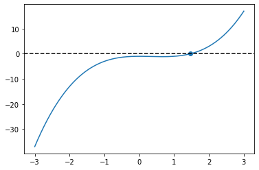
Exercise 07.2:
def f(x):
    return x**3 - x**2 - 1.0

x = np.linspace(-3.0, 3.0, 1000)
root = bisection(f, np.min(x), np.max(x))
print(root)

fig, ax = plt.subplots()
ax.plot(x, f(x))
ax.scatter(root, f(root))
ax.axhline(0.0, color="black", linestyle="--")
plt.show()
root found within tolerance 1e-15 using 53 iterations
1.4655712318767677
Exercise 07.3:
def secant_method(f, x_0, x_1, error_tolerance=1.0e-15, max_iterations=500):
    """
    Finds the root of a continuous function using secant method.
    Args:
        f (function): Continuous function
        x_0 (float): First initial guess
        x_1 (float): Second initial guess
        error_tolerance (float): Error tolerance
        max_iterations (int): Maximum number of iterations
    Returns:
        float: The root of function f
    Raises:
        RuntimeError: Raises an exception when the root is not found
    """
    k = 0
    while k < max_iterations:
        x = (f(x_1) * x_0 - f(x_0) * x_1) / (f(x_1) - f(x_0))
        x_0 = x_1
        x_1 = x
        k = k + 1
        if np.abs(x_1 - x_0) < error_tolerance:
            #print("root found within tolerance", error_tolerance, "using", k, "iterations")
            return x
    raise RuntimeError("no root found within tolerance", error_tolerance, "using", max_iterations, "iterations")
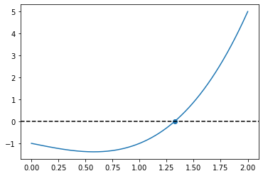
Exercise 07.4:
def f(x):
    return x**3 - x - 1.0

x = np.linspace(0.0, 2.0, 1000)
root = secant_method(f, np.min(x), np.max(x))
print(root)

fig, ax = plt.subplots()
ax.plot(x, f(x))
ax.scatter(root, f(root))
ax.axhline(0.0, color="black", linestyle="--")
plt.show()
1.3247179572447458
Exercise 07.5:
def false_position_method(f, x_0, x_1, error_tolerance=1.0e-15, max_iterations=500):
    """
    Finds the root of a continuous function using false position method.
    Args:
        f (function): Continuous function defined on an interval [x_0, x_1], where f(x_0) and f(x_1) have opposite signs
        x_0 (float): Leftmost point of the interval
        x_1 (float): Rightmost point of the interval
        error_tolerance (float): Error tolerance
        max_iterations (int): Maximum number of iterations
    Returns:
        float: The root of function f
    Raises:
        RuntimeError: Raises an exception when the root is not found
    """
    k = 0
    while k < max_iterations:
        x = (f(x_1) * x_0 - f(x_0) * x_1) / (f(x_1) - f(x_0))
        if f(x_0) * f(x) > 0:
            x_0 = x
        else:
            x_1 = x
        k = k + 1
        if np.abs(f(x)) < error_tolerance:
            #print("root found within tolerance", error_tolerance, "using", k, "iterations")
            return x
    raise RuntimeError("no root found within tolerance", error_tolerance, "using", max_iterations, "iterations")
Exercise 07.6:
def newton_raphson(f, x_0, error_tolerance=1.0e-15, max_iterations=500):
    """
    Finds the solution of one nonlinear eqution using Newton-Raphson method.
    Args:
        f (function): Function whose derivative is continuous and nonzero in the neighborhood of a root
        x_0 (float): Initial guess
        error_tolerance (float): Error tolerance
        max_iterations (int): Maximum number of iterations
    Returns:
        float: The solution of a given equation
    Raises:
        RuntimeError: Raises an exception when the solution is not found
    """
    def df_dx(f, x, h=1.0e-7):
        return (f(x + h) - f(x)) / h
    k = 0
    while k < max_iterations:
        x = x_0 - f(x_0) / df_dx(f, x_0)
        k = k + 1
        if np.abs(f(x)) < error_tolerance:
            #print("root found within tolerance", error_tolerance, "using", k, "iterations")
            return x
        x_0 = x
    raise RuntimeError("no root found within tolerance", error_tolerance, "using", max_iterations, "iterations")
Exercise 07.7:
def f(x):
    return x**3 - np.cos(x)

root = newton_raphson(f, 0.0)
print(root)
0.8654740331016145
Exercise 07.8:
def f(x):
    return x**(1/3) + 2.0
try:
    root = newton_raphson(f, 0.0)
except Exception as e:
    print(e)
else:
    print(root)
complex division by zero
Exercise 07.9:
def newton_raphson_2d(f_0, f_1, x_0, y_0, error_tolerance=1.0e-15, max_iterations=500):
    """
    Finds the solution of a sytem of two equations using Newton-Raphson method.
    Args:
        f_1 (function): Function whose derivative is continuous and nonzero in the neighborhood of a root
        f_2 (function): Function whose derivative is continuous and nonzero in the neighborhood of a root
        x_0 (float): Initial guess
        y_0 (float): Initial guess
        error_tolerance (float): Error tolerance
        max_iterations (int): Maximum number of iterations
    Returns:
        list: The vector of solution of a given sytem of equations
    Raises:
        RuntimeError: Raises an exception when the solution is not found
    """
    def df_dx(f, x, y, h=1.0e-7):
        return (f(x + h, y) - f(x, y)) / h
    def df_dy(f, x, y, h=1.0e-7):
        return (f(x, y + h) - f(x, y)) / h
    k = 0
    J = np.zeros((2, 2))
    b = np.zeros(2)
    while k < max_iterations:
        J[0][0] = df_dx(f_0, x_0, y_0)
        J[0][1] = df_dy(f_0, x_0, y_0)
        J[1][0] = df_dx(f_1, x_0, y_0)
        J[1][1] = df_dy(f_1, x_0, y_0)
        b[0] = -f_0(x_0, y_0)
        b[1] = -f_1(x_0, y_0)
        delta = linalg.solve(J, b)
        x = x_0 + delta[0]
        y = y_0 + delta[1]
        k = k + 1
        if np.max([np.abs(f_0(x, y)), np.abs(f_1(x, y))]) < error_tolerance:
            #print("root found within tolerance", error_tolerance, "using", k, "iterations")
            return [x, y]
        x_0 = x
        y_0 = y
    raise RuntimeError("no root found within tolerance", error_tolerance, "using", max_iterations, "iterations")
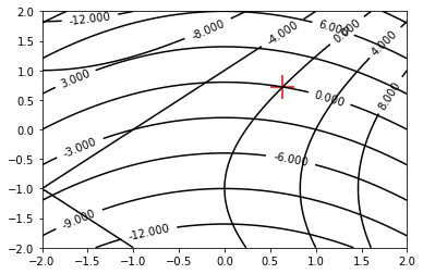
Exercise 07.10:
def f_0(x, y):
    return x**2 + 4.0 * x - y**2 - 2.0 * y - 1.0

def f_1(x, y):
    return x**2 + 5*y - 4.0

root = newton_raphson_2d(f_0, f_1, 0.0, 0.0)
print(root)

x = np.linspace(-2.0, 2.0, 100)
y = np.linspace(-2.0, 2.0, 100)
X, Y = np.meshgrid(x, y)

fig, ax = plt.subplots()
ax.scatter(root[0], root[1], 500, marker="+", color="red")
a = ax.contour(X, Y, f_0(X, Y), colors="black", linestyles="-")
b = ax.contour(X, Y, f_1(X, Y), colors="black", linestyles="-")
ax.clabel(a)
ax.clabel(b)
plt.show()
[0.6371078452969544, 0.7188187186922144]
Exercise 08.1:
def golden_section_search(f, a, b, error_tolerance=1.0e-15, max_iterations=500):
    """
    Finds the minimum of function using golden section search.
    Args:
        f (function): A strictly unimodal function on [a, b]
        a (float): Left endpoint of the interval
        b (float): Right endpoint of the interval
        error_tolerance (float): Error tolerance
        max_iterations (int): Maximum number of iterations
    Returns:
        float: A coordinate of minimum
    Raises:
        RuntimeError: Raises an exception when the minimum is not found
    """
    gr = (np.sqrt(5.0) + 1.0) / 2.0
    k = 0
    c = a + (b - a) / gr
    d = b - (b - a) / gr
    while k <= max_iterations:
        if f(c) < f(d):
            a = d
            d = c
            c = a + (b - a) / gr
        else:
            b = c
            c = d
            d = b - (b - a) / gr
        k = k + 1
        if np.abs(b - a) < error_tolerance:
            print("minimum found within tolerance", error_tolerance, "using", k, "iterations")
            return (a + b) / 2.0
    raise RuntimeError("minimum not found within tolerance", error_tolerance, "using", max_iterations, "iterations")
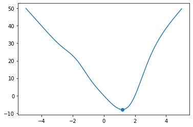
Exercise 08.2:
def f(x):
    return 3.0 * np.sin(x + 2) + x**2 - 3.0 * x + 5.0

x = np.linspace(-5.0, 5.0, 1000)

x_min = golden_section_search(f, np.min(x), np.max(x), 1.0e-7)
print(x_min)

fig, ax = plt.subplots()
ax.plot(x, f(x))
ax.scatter(x_min, f(x_min))
plt.show()
minimum found within tolerance 1e-07 using 39 iterations
2.215301416536189
Exercise 08.3:
def parabolic_interpolation_search(f, a, b, c, error_tolerance=1.0e-15, max_iterations=500):
    """
    Finds the minimum of function using parabolic interpolation search.
    Args:
        f (function): A strictly unimodal function on [a, b]
        a (float): Left endpoint of the interval
        b (float): Point inside the interval
        c (float): Right endpoint of the interval
        error_tolerance (float): Error tolerance
        max_iterations (int): Maximum number of iterations
    Returns:
        float: A coordinate of minimum
    Raises:
        RuntimeError: Raises an exception when the minimum is not found
    """
    k = 0
    while k <= max_iterations:
        x_min = b - 0.5 * ((b - a)**2 * (f(b) - f(c)) - (b - c)**2 * (f(b) - f(a))) / ((b - a)
                * (f(b) - f(c)) - (b - c) * (f(b) - f(a)))
        if x_min < b:
            if f(x_min) < f(b):
                c = b
                b = x_min
            else:
                a = x_min
        else:
            if f(x_min) < f(b):
                a = b
                b = x_min
            else:
                c = x_min
        k = k + 1
        if np.abs(c - a) < error_tolerance:
            #print("minimum found within tolerance", error_tolerance, "using", k, "iterations")
            return b
    raise RuntimeError("minimum not found within tolerance", error_tolerance, "using", max_iterations, "iterations")
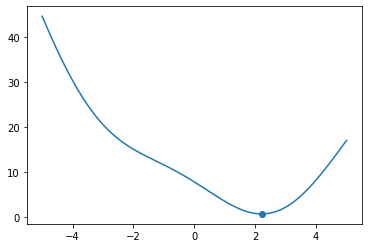
Exercise 08.4:
def f(x):
    return np.log(1.0 + np.abs(x - 1)**2) - np.arctan(x)

x = np.linspace(-5.0, 5.0, 1000)

x_min = parabolic_interpolation_search(f, np.min(x), (np.min(x) + np.max(x)) / 2.0, np.max(x), 1.0e-7)
print(x_min)

fig, ax = plt.subplots()
ax.plot(x, f(x))
ax.scatter(x_min, f(x_min))
plt.show()
1.211659172323886
Exercise 08.5:
def steepest_descent(f, x_0, step, error_tolerance=1.0e-15, max_iterations=1e5):
    """
    Finds the minimum of function using the method of steepest descent.
    Args:
        f (function): A strictly unimodal and differentiable function in a neighborhood of a point x_0
        x_0 (float): Initial guess
        step (float): Step size multiplier
        error_tolerance (float): Error tolerance
        n_max (int): Maximum number of iterations
    Returns:
        float: A coordinate of minimum
    Raises:
        RuntimeError: Raises an exception when the minimum is not found
    """
    def grad(f, x, h=1.0e-8):
        return (f(x + h) - f(x)) / h
    k = 0
    while k < max_iterations:
        x_1 = x_0 - step * grad(f, x_0)
        k = k + 1
        if np.abs(x_1 - x_0) < error_tolerance:
            #print("minimum found within tolerance", error_tolerance, "using", k, "iterations")
            return x_1
        x_0 = x_1
    raise RuntimeError("minimum not found within tolerance", error_tolerance, "using", max_iterations, "iterations")
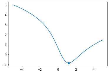
Exercise 08.6:
def f(x):
    return -x**3 * np.exp(-(x + 1)**2) + 10 * x * np.tanh(x - 2)

x = np.linspace(-5, 5, 1000)

x_min = steepest_descent(f, 0.0, 1.0e-3, 1.0e-7)
print(x_min)

fig, ax = plt.subplots()
ax.plot(x, f(x))
ax.scatter(x_min, f(x_min))
plt.show()
1.1952907012523994
Exercise 08.7:
def steepest_descent_nd(f, x_0, step, error_tolerance=1.0e-15, max_iterations=1e5):
    """
    Finds the minimum of function using the method of steepest descent.
    Args:
        f (function): A strictly unimodal and differentiable function in a neighborhood of a point x_0
        x_0 (float): Initial guess
        step (float): Step size multiplier
        error_tolerance (float): Error tolerance
        n_max (int): Maximum number of iterations
    Returns:
        float: A coordinate of minimum
    Raises:
        RuntimeError: Raises an exception when the minimum is not found
    """
    def grad(f, x, h=1.0e-8):
        return np.array([(f(x + h * np.identity(x.size)[j]) - f(x)) / h for j in range(x.size)])
    k = 0
    while k < max_iterations:
        x_1 = x_0 - step * grad(f, x_0)
        k = k + 1
        if linalg.norm(x_1 - x_0) < error_tolerance:
            print("minimum found within tolerance", error_tolerance, "using", k, "iterations")
            return x_1
        x_0 = x_1
    raise RuntimeError("minimum not found within tolerance", error_tolerance, "using", max_iterations, "iterations")
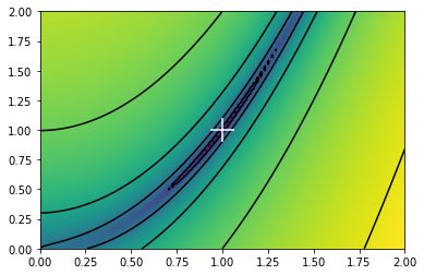
Exercise 08.8:
def f(x):
    return (1.0 - x[0])**2.0  + 100.0 * (x[1] - x[0]**2.0)**2.0

x = np.meshgrid(np.linspace(0.0, 2.0, 100), np.linspace(0.0, 2.0, 100))

x_min = steepest_descent_nd(f, np.array([0.0, 0.0]), 1.0e-3, 1.0e-7)
print(x_min)

fig, ax = plt.subplots()
ax.pcolormesh(x[0], x[1], f(x), norm=mpl.colors.LogNorm(), shading="gouraud", zorder=0)
ax.contour(x[0], x[1], f(x), norm=mpl.colors.LogNorm(), colors="black", linestyles="-", zorder=1)
ax.scatter(x_min[0], x_min[1], color="white", marker="+", s=500, zorder=2)
plt.show()
minimum found within tolerance 1e-07 using 19777 iterations
[0.99988525 0.99977007]
Exercise 09.1:
def midpoint_rule(f, a, b, N=100):
    """
    Calculates definite integral of 1D function using rectangular rule.
    Args:
        f (function): A function defined on interval [a, b]
        a (float): Left-hand side point of the interval
        b (float): Right-hand side point of the interval
        N (int): Number of subdivisions of the interval [a, b]
    Returns:
        float: Definite integral
    """
    x, h = np.linspace(a, b, N, retstep=True)
    I = 0.0
    for i in range(N - 1):
        I += h * f((x[i] + x[i+1]) / 2.0)
    return I
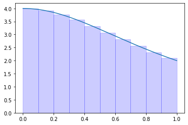
Exercise 09.2:
def f(x):
    return 4.0 / (1.0 + x**2)

a = 0.0
b = 1.0
N = 10

I = midpoint_rule(f, a, b, N)
error = np.abs(np.pi - I)
print(I, error)

if error < 1.0e-5:
    print(True)
else:
    print(False)

x = np.linspace(a, b, 1000)
t = np.linspace(a, b, N + 1)

fig, ax = plt.subplots()
ax.plot(x, f(x))
for i in range(N):
    x_s = np.array([(t[i] + t[i+1]) / 2.0])
    y_s = f(x_s)
    l = interpolate.lagrange(x_s, y_s)
    xx = np.linspace(t[i], t[i+1], 10)
    ax.stackplot(xx, l(xx), color="blue", alpha=0.2)
plt.show()
3.142621456557612 0.0010288029678187094
False
Exercise 09.3:
def trapezoidal_rule(f, a, b, N=100):
    """
    Calculates definite integral of 1D function using trapezoidal rule.
    Args:
        f (function): A function defined on interval [a, b]
        a (float): Left-most point of the interval
        b (float): Right-most point of the interval
        N (int): Number of subdivisions of the interval [a, b]
    Returns:
        float: Definite integral
    """
    x, h = np.linspace(a, b, N, retstep=True)
    I = 0.0
    for i in range(N - 1):
        I += h / 2.0 * (f(x[i]) + f(x[i+1]))
    return I
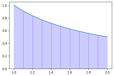
Exercise 09.4:
def f(x):
    return 1.0 / x

a = 1.0
b = 2.0
N = 10

I = trapezoidal_rule(f, a, b, N)
error = np.abs(np.log(2) - I)
print(I, error)

if error < 1.0e-5:
    print(True)
else:
    print(False)

x = np.linspace(a, b, 1000)
t = np.linspace(a, b, N + 1)

fig, ax = plt.subplots()
ax.plot(x, f(x))
for i in range(N):
    x_s = np.array([t[i], t[i+1]])
    y_s = f(x_s)
    l = interpolate.lagrange(x_s, y_s)
    xx = np.linspace(t[i], t[i+1], 10)
    ax.stackplot(xx, l(xx), color="blue", alpha=0.2)
plt.show()
0.6939176020058372 0.0007704214458919001
False
Exercise 09.5:
def simpsons_quadratic_rule(f, a, b, N=100):
    """
    Calculates definite integral of 1D function using Simpson's 1/3 rule.
    Args:
        f (function): A function defined on interval [a, b]
        a (float): Left-hand side point of the interval
        b (float): Right-hand side point of the interval
        N (int): Number of subdivisions of the interval [a, b]
    Returns:
        float: Definite integral
    """
    x, h = np.linspace(a, b, N, retstep=True)
    I = 0.0
    for i in range(N - 2):
        I += h * (1.0 / 6.0 * f(x[i]) + 2.0 / 3.0 * f((x[i] + x[i+1]) / 2.0) + 1.0 / 6.0 * f(x[i+1]))
    return I
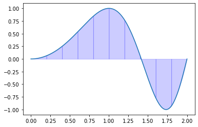
Exercise 09.6:
def f(x):
    return np.sin(np.pi * x**2 / 2.0)

a = 0.0
b = 2.0
N = 10

I = simpsons_quadratic_rule(f, a, b, N)
error = np.abs(special.fresnel(2)[0] - I)
print(I, error)

if error < 1.0e-5:
    print(True)
else:
    print(False)

x = np.linspace(a, b, 1000)
t = np.linspace(a, b, N + 1)

fig, ax = plt.subplots()
ax.plot(x, f(x))
for i in range(N):
    x_s = np.array([t[i], (t[i] + t[i+1]) / 2.0, t[i+1]])
    y_s = f(x_s)
    l = interpolate.lagrange(x_s, y_s)
    xx = np.linspace(t[i], t[i+1], 10)
    ax.stackplot(xx, l(xx), color="blue", alpha=0.2)
plt.show()
0.47206995069497343 0.1286542723312752
False
Exercise 09.7:
def simpsons_cubic_rule(f, a, b, n=100):
    """
    Calculates definite integral of 1D function using Simpson's 3/8 rule.
    Args:
        f (function): A function defined on interval [a, b]
        a (float): Left-hand side point of the interval
        b (float): Right-hand side point of the interval
        n (int): Number of subdivisions of the interval [a, b]
    Returns:
        float: Definite integral
    """
    x, h = np.linspace(a, b, n, retstep=True)
    I = 0
    for i in range(n-1):
        I += h * (1.0 / 8.0 * f(x[i]) + 3.0 / 8.0 * f((2.0 * x[i] + x[i+1]) / 3.0) \
            + 3.0 / 8.0 * f((x[i] + 2.0 * x[i+1]) / 3.0) + 1.0 / 8.0 * f(x[i+1]))
    return I
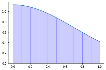
Exercise 09.8:
def f(x):
    return 2.0 / np.sqrt(np.pi) * np.exp(-x**2)

a = 0.0
b = 1.0
N = 10

I = simpsons_cubic_rule(f, a, b, N)
error = np.abs(special.erf(1) - I)
print(I, error)

if error < 1.0e-5:
    print(True)
else:
    print(False)

x = np.linspace(a, b, 1000)
t = np.linspace(a, b, N + 1)

fig, ax = plt.subplots()
ax.plot(x, f(x))
for i in range(N):
    x_s = np.array([t[i], (2.0 * t[i] + t[i+1]) / 3.0, (t[i] + 2.0 * t[i+1]) / 3.0, t[i+1]])
    y_s = f(x_s)
    l = interpolate.lagrange(x_s, y_s)
    xx = np.linspace(t[i], t[i+1], 10)
    ax.stackplot(xx, l(xx), color="blue", alpha=0.2)
plt.show()
0.8427008319786382 3.902892342644293e-08
True
Exercise 09.9:
def rombergs_method(f, a, b, m=10):
    """
    Calculates definite integral of 1D function using Romberg's method.
    Args:
        f (function): A function defined on interval [a, b]
        a (float): Left-hand side point of the interval
        b (float): Right-hand side point of the interval
        m (int): Number of extrapolations
    Returns:
        float: Definite integral
    """
    R = np.zeros((m, m))
    R[0, 0] = trapezoidal_rule(f, a, b, 2)
    for k in range(1, m):
        R[k, 0] = trapezoidal_rule(f, a, b, 2**k + 1)
        for j in range(1, k + 1):
            R[k, j] = R[k, j-1] + 1.0 / (4.0**j - 1.0) * (R[k, j-1] - R[k-1, j-1])
    return R[m-1, m-1]
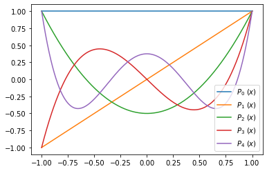
Exercise 09.10:
def legendre_polynomial(n):
    """
    Calculates a Legendre polynomial of degree n using recursive formula.
    Args:
        n (int): Degree of the polynomial
    Returns:
        numpy.poly1d: The Legendre polynomial of degree n
    """
    P = [0 for i in range(n + 1)]
    for i in range(n + 1):
        if i == 0:
            P[i] = np.poly1d(1)
        elif i == 1:
            P[i] = np.poly1d([1, 0])
        else:
            P[i] = (2.0 * i - 1.0) / i * np.poly1d([1, 0]) * P[i-1] - (i - 1.0) / i * P[i-2]
    return P[n]
Exercise 09.11:
x = np.linspace(-1.0, 1.0, 1000)

fig, ax = plt.subplots()
for i in range(5):
    P = legendre_polynomial(i)
    ax.plot(x, P(x), label=r"$ P_{} \ (x) $".format(i))
ax.legend()
plt.show()
Exercise 09.12:
def gauss_legendre_quadrature(f, a, b, N=3):
    """
    Calculates definite integral of 1D function using Gaussian quadrature rule.
    Args:
        f (function): A function defined on interval [a, b]
        a (float): Left-hand side point of the interval
        b (float): Right-hand side point of the interval
        N (int): Degree of used polynomial
    Returns:
        float: Definite integral
    """
    x, w = np.polynomial.legendre.leggauss(N)
    I = 0.0
    for i in range(N):
        I += w[i] * f((b - a) / 2.0 * x[i] + (a + b) / 2.0)
    return (b - a) / 2.0 * I
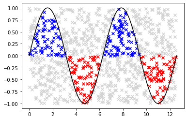
Exercise 09.13:
def monte_carlo_integration(f, a, b, c, d, N=500):
    """
    Calculates definite integral of 1D function using Monte Carlo method.
    Args:
        f (function): A function defined on interval [a, b]
        a (float): Left-hand side point of the interval
        b (float): Right-hand side point of the interval
        N (int): Number of random points generated
    Returns:
        float: Definite integral
    """
    x = np.linspace(a, b, 1000)
    fig, ax = plt.subplots()
    ax.plot(x, f(x), color="black")
    S = 0
    for i in range(N):
        x_p = np.random.uniform(a, b)
        y_p = np.random.uniform(c, d)
        if y_p <= f(x_p) and y_p >= 0.0:
            S = S + 1
            ax.scatter(x_p, y_p, marker="x", color='blue')
        elif y_p >= f(x_p) and y_p <= 0.0:
            S = S - 1
            ax.scatter(x_p, y_p, marker="x", color='red')
        else:
            ax.scatter(x_p, y_p, marker="x", color='lightgray')
    return (S / N) * (b - a) * (d - c)
Exercise 09.14:
def f(x):
    return np.sin(x)

I = monte_carlo_integration(f, 0.0, 4.0 * np.pi, -1.0, 1.0, 1000)
error = np.abs(0.0 - I)
print(I, error)
0.20106192982974677 0.20106192982974677
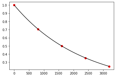
Exercise 10.1:
def forward_euler(f, x_0, x_n, y_0, n): # Runge-Kutta 1st order method
    x, h = np.linspace(x_0, x_n, n, retstep=True)
    y = np.zeros(n)
    y[0] = y_0
    for i in range(n-1):
        y[i+1] = y[i] + h * f(x[i], y[i])
    return x, y
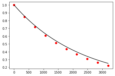
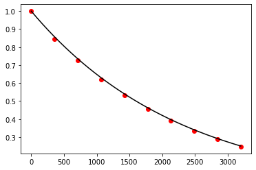
Exercise 10.2:
def f(t, N):
    return -np.log(2.0) / 1600.0 * N

t, N = forward_euler(f, 0.0, 3200.0, 1.0, 10)

t_exact = np.linspace(0.0, 3200.0, 1000)
N_exact = 1.0 * np.exp(-np.log(2.0) / 1600.0 * t_exact)

fig, ax = plt.subplots()
ax.plot(t_exact, N_exact, color='black')
ax.scatter(t, N, color='red')
plt.show()
Exercise 10.3:
def runge_kutta_2(f, x_0, x_n, y_0, n):
    x, h = np.linspace(x_0, x_n, n, retstep=True)
    y = np.zeros(n)
    y[0] = y_0
    for i in range(n-1):
        k_1 = f(x[i], y[i])
        #k_2 = f(x[i] + h / 2.0, y[i] + h / 2.0 * k_1)
        #y[i+1] = y[i] + h * k_2 # rectangular rule
        k_2 = f(x[i] + h, y[i] + h * k_1)
        y[i+1] = y[i] + h / 2.0 * (k_1 + k_2) # trapezoid rule (Heun's predictor-corrector method)
    return x, y
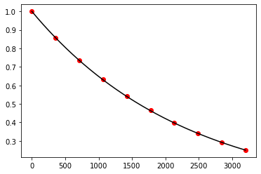
Exercise 10.4:
def f(t, N):
    return -np.log(2.0) / 1600.0 * N

t, N = runge_kutta_2(f, 0.0, 3200.0, 1.0, 10)

t_exact = np.linspace(0.0, 3200.0, 1000)
N_exact = 1.0 * np.exp(-np.log(2.0) / 1600.0 * t_exact)

fig, ax = plt.subplots()
ax.plot(t_exact, N_exact, color='black')
ax.scatter(t, N, color='red')
plt.show()
Exercise 10.5:
def runge_kutta_3(f, x_0, x_n, y_0, n):
    x, h = np.linspace(x_0, x_n, n, retstep=True)
    y = np.zeros(n)
    y[0] = y_0
    for i in range(n-1):
        k_1 = f(x[i], y[i])
        k_2 = f(x[i] + h / 2.0, y[i] + h / 2.0 * k_1)
        k_3 = f(x[i] + h, y[i] + h * (-k_1 + 2.0 * k_2))
        y[i+1] = y[i] + h * (k_1 / 6.0 + 2.0 * k_2 / 3.0 + k_3 / 6.0) # Simpson's 1/3 rule
    return x, y
Exercise 10.6:
def f(t, N):
    return -np.log(2.0) / 1600.0 * N

t, N = runge_kutta_3(f, 0.0, 3200.0, 1.0, 10)

t_exact = np.linspace(0.0, 3200.0, 1000)
N_exact = 1.0 * np.exp(-np.log(2.0) / 1600.0 * t_exact)

fig, ax = plt.subplots()
ax.plot(t_exact, N_exact, color='black')
ax.scatter(t, N, color='red')
plt.show()

Exercise 10.7:
def runge_kutta_4(f, x_0, x_n, y_0, n):
    x, h = np.linspace(x_0, x_n, n, retstep=True)
    y = np.zeros(n)
    y[0] = y_0
    for i in range(n-1):
        k_1 = f(x[i], y[i])
        k_2 = f(x[i] + h / 2.0, y[i] + h / 2.0 * k_1)
        k_3 = f(x[i] + h / 2.0, y[i] + h / 2.0 * k_2)
        k_4 = f(x[i] + h, y[i] + h * k_3)
        y[i+1] = y[i] + h / 6.0 * (k_1 + 2.0 * k_2 + 2.0 * k_3 + k_4)
        #k_2 = f(x[i] + h / 3.0, y[i] + h / 3.0 * k_1)
        #k_3 = f(x[i] + 2.0 * h / 3.0, y[i] + h * (-k_1 / 3.0 + k_2))
        #k_4 = f(x[i] + h, y[i] + h * (k_1 - k_2 + k_3))
        #y[i+1] = y[i] + h * (k_1 / 8.0 + 3.0 * k_2 / 8.0 + 3.0 * k_3 / 8.0 + k_4 / 8.0) # Simpson's 3/8 rule
    return x, y
Exercise 10.8:
def f(t, N):
    return -np.log(2.0) / 1600.0 * N

t, N = runge_kutta_4(f, 0.0, 3200.0, 1.0, 10)

t_exact = np.linspace(0.0, 3200.0, 1000)
N_exact = 1.0 * np.exp(-np.log(2.0) / 1600.0 * t_exact)

fig, ax = plt.subplots()
ax.plot(t_exact, N_exact, color='black')
ax.scatter(t, N, color='red')
plt.show()

Exercise 10.9:
def backward_euler(f, x_0, x_n, y_0, n): # implicit method
    x, h = np.linspace(x_0, x_n, n, retstep=True)
    y = np.zeros(n)
    y[0] = y_0
    for i in range(n-1):
        y[i+1] = optimize.fsolve(lambda z: z - y[i] - h * f(x[i+1], z), y[i])
    return x, y
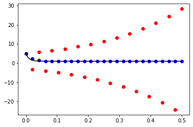
Exercise 10.10:
def f(x, y):
    return -100.0 * y + 100.0

y0 = 5.0

x_1, y_1 = forward_euler(f, 0.0, 0.5, y0, 25)
x_2, y_2 = backward_euler(f, 0.0, 0.5, y0, 25)

x_exact = np.linspace(0.0, 0.5, 1000)
y_exact = (y0 - 1.0) * np.exp(-100.0 * x_exact) + 1.0

fig, ax = plt.subplots()
ax.plot(x_exact, y_exact, color='black')
ax.scatter(x_1, y_1, color='red')
ax.scatter(x_2, y_2, color='blue')
plt.show()
Exercise 10.11:
def leap_frog(f, x_0, x_n, y_0, n):
x, h = np.linspace(x_0, x_n, n, retstep=True)
y = np.zeros(n)
y[0] = y_0
y[1] = y[0] + h * f(x[0], y[0])
for i in range(1, n-1):
y[i+1] = y[i-1] + 2.0 * h * f(x[i], y[i])
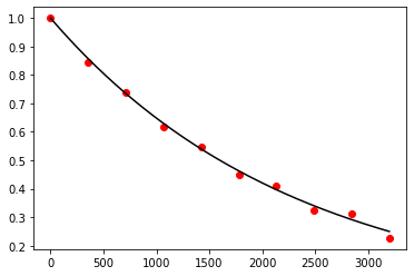
return x, y
Exercise 10.12:
def f(t, N):
    return -np.log(2.0) / 1600.0 * N

t, N = leap_frog(f, 0.0, 3200.0, 1.0, 10)

t_exact = np.linspace(0.0, 3200.0, 1000)
N_exact = 1.0 * np.exp(-np.log(2.0) / 1600.0 * t_exact)

fig, ax = plt.subplots()
ax.plot(t_exact, N_exact, color='black')
ax.scatter(t, N, color='red')
plt.show()
Exercise 10.13:
def adams_bashforth(f, x_0, x_n, y_0, n):
    x, h = np.linspace(x_0, x_n, n, retstep=True)
    y = np.zeros(n)
    y[0] = y_0
    y[1] = y[0] + h * f(x[0], y[0])
    for i in range(1, n-1):
        y[i+1] = y[i] + 3.0 / 2.0 * h * f(x[i], y[i]) - 1.0 / 2.0 * h * f(x[i-1], y[i-1])
    return x, y
Exercise 10.14:
def f(t, N):
    return -np.log(2.0) / 1600.0 * N

t, N = adams_bashforth(f, 0.0, 3200.0, 1.0, 10)

t_exact = np.linspace(0.0, 3200.0, 1000)
N_exact = 1.0 * np.exp(-np.log(2.0) / 1600.0 * t_exact)

fig, ax = plt.subplots()
ax.plot(t_exact, N_exact, color='black')
ax.scatter(t, N, color='red')
plt.show()

Exercise 10.15:
def adams_moulton(f, x_0, x_n, y_0, n):
    x, h = np.linspace(x_0, x_n, n, retstep=True)
    y = np.zeros(n)
    y[0] = y_0
    y[1] = y[0] + h * f(x[0], y[0])
    for i in range(1, n-1):
        y[i+1] = optimize.fsolve(lambda z: z - y[i] - h * (5.0 / 12.0 * f(x[i+1], z) + 2.0 / 3.0 * \
            f(x[i], y[i]) - 1.0 / 12.0 * f(x[i-1], y[i-1])), y[i])
    return x, y
Exercise 10.16:
def f(t, N):
    return -np.log(2.0) / 1600.0 * N

t, N = adams_moulton(f, 0.0, 3200.0, 1.0, 10)

t_exact = np.linspace(0.0, 3200.0, 1000)
N_exact = 1.0 * np.exp(-np.log(2.0) / 1600.0 * t_exact)

fig, ax = plt.subplots()
ax.plot(t_exact, N_exact, color='black')
ax.scatter(t, N, color='red')
plt.show()

Exercise 10.17:
def predictor_corrector(f, x_0, x_n, y_0, n):
    x, h = np.linspace(x_0, x_n, n, retstep=True)
    y = np.zeros(n)
    y[0] = y_0
    y[1] = y[0] + h * f(x[0], y[0])
    for i in range(1, n-1):
        q = y[i] + 3.0 / 2.0 * h * f(x[i], y[i]) - 1.0 / 2.0 * h * f(x[i-1], y[i-1])
        y[i+1] = y[i] + h * (5.0 / 12.0 * f(x[i+1], q) + 2.0 / 3.0 * f(x[i], y[i]) - 1.0 / 12.0 * f(x[i-1], y[i-1]))
    return x, y
Exercise 10.18:
def f(t, N):
    return -np.log(2.0) / 1600.0 * N

t, N = predictor_corrector(f, 0.0, 3200.0, 1.0, 10)

t_exact = np.linspace(0.0, 3200.0, 1000)
N_exact = 1.0 * np.exp(-np.log(2.0) / 1600.0 * t_exact)

fig, ax = plt.subplots()
ax.plot(t_exact, N_exact, color='black')
ax.scatter(t, N, color='red')
plt.show()
Exercise 10.19:
def bulirsch_stoer(f, x_0, x_n, y_0, n, m=5):
    x = np.linspace(x_0, x_n, n)
    y = np.zeros(n)
    y[0] = y_0
    for i in range(n-1):
        T = np.zeros((m, m))
        T[0, 0] = leap_frog(f, x[i], x[i+1], y[i], 2)[1][-1]
        for k in range(1, m):
            T[k, 0] = leap_frog(f, x[i], x[i+1], y[i], 2 * (k+1))[1][-1]
            for j in range(1, k+1):
                T[k, j] = T[k, j-1] + 1.0 / (4**j - 1) * (T[k, j-1] - T[k-1, j-1])
        y[i+1] = T[m-1, m-1]
    return x, y
Exercise 10.20:
def f(t, N):
    return -np.log(2.0) / 1600.0 * N

t, N = bulirsch_stoer(f, 0.0, 3200.0, 1.0, 5, 4)

t_exact = np.linspace(0.0, 3200.0, 1000)
N_exact = 1.0 * np.exp(-np.log(2.0) / 1600.0 * t_exact)

fig, ax = plt.subplots()
ax.plot(t_exact, N_exact, color='black')
ax.scatter(t, N, color='red')
plt.show()
Exercise 11.1:
def shooting_method(f, g, a, b, n, alpha, beta):
    """
    Solves 2nd order explicit ODE in the form y(x)'' = f(x, y(x), y(x)') in [a, b] with y(a) = alpha, y(b) = beta
    using shooting method.
    Args:
        f (function): function
        g (function): function
        a (float): The left-most point of the interval
        b (float): The right-most point of the interval
        n (int): number of points dividing interval [a, b]
        alpha (float): initial value at x = a
        beta (float): initial value at x = b
    Returns:
        numpy.ndarray: Vector of grid-points
        numpy.ndarray: Vector of solution
    """
    def semi_implicit_euler_system(f, g, a, b, n, y_0, z_0):
        x, h = np.linspace(a, b, n, retstep=True)
        y = np.zeros(n)
        z = np.zeros(n)
        y[0] = y_0
        z[0] = z_0
        for i in range(n - 1):
            z[i + 1] = z[i] + h * f(x[i], y[i], z[i])
            y[i + 1] = optimize.fsolve(lambda q: q - y[i] - h * g(x[i + 1], q, z[i + 1]), y[i])
        return x, y
    def shooting_function(gamma):
        x, y = semi_implicit_euler_system(f, g, a, b, n, alpha, gamma)
        return y[-1] - beta
    root = optimize.fsolve(shooting_function, 0.0)
    x, y = semi_implicit_euler_system(f, g, a, b, n, alpha, root)
    return x, y
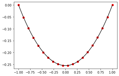
Exercise 11.2:
def f(x, y, z):
    return 0.5 * np.sqrt(1.0 + z**2)

def g(x, y, z):
    return z

a = -1.0
b = 1.0
n = 20
alpha = 0.0
beta = 0.0

x_numerical, y_numerical = shooting_method(f, g, a, b, n, alpha, beta)

x_analytical = np.linspace(a, b, 100)
y_analytical = 2.0 * np.cosh(x_analytical / 2.0) - 2.255

fig, ax = plt.subplots()
ax.scatter(x_numerical, y_numerical, color="red")
ax.plot(x_analytical, y_analytical, color="black")
plt.show()
Exercise 11.3:
def finite_difference_method(a, b, n, p, q, r, s, alpha, beta):
    """
    Solves 2nd order linear ODE in the form p(x)y(x)'' + q(x)y(x)' + r(x)y(x) + s(x) = 0 in [a, b] with y(a) = alpha,
    y(b) = beta using finite difference method.
    Args:
        a (float): The left-most point of the interval
        b (float): The right-most point of the interval
        n (int): Number of points dividing interval [a, b]
        p (function): Arbitrary differentiable function
        q (function): Arbitrary differentiable function
        r (function): Arbitrary differentiable function
        s (function): Arbitrary differentiable function
        alpha (float): Initial value at x = a
        beta (float): Initial value at x = b
    Returns:
        numpy.ndarray: Vector of grid-points
        numpy.ndarray: Vector of solution
    """
    x, h = np.linspace(a, b, n, retstep=True)
    A = np.zeros((n, n))
    b = np.zeros(n)
    for i in range(n):
        if i == 0:
            A[i, i] = 1.0
            b[i] = alpha
        elif i == n - 1:
            A[i, i] = 1.0
            b[i] = beta
        else:
            A[i, i - 1] = p(x[i])
            A[i, i] = -2.0 * p(x[i]) -q(x[i]) * h + r(x[i]) * h**2
            A[i, i + 1] = p(x[i]) + q(x[i]) * h
            b[i] = -s(x[i]) * h**2
    y = linalg.solve(A, b)
    return x, y
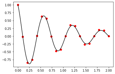
Exercise 11.4:
p = lambda x: 1.0
q = lambda x: 2.0
r = lambda x: 100.0
s = lambda x: 0.0

a = 0.0
b = 2.0
n = 20
alpha = 1.0
beta = 0.0

t_numerical, y_numerical = finite_difference_method(a, b, n, p, q, r, s, alpha, beta)

t_analytical = np.linspace(a, b, 100)
y_analytical = -np.exp(-t_analytical) * np.sin(3.0 * np.sqrt(11.0) * (t_analytical - 2.0)) / np.sin(6.0 * np.sqrt(11.0))

# plot results
fig, ax = plt.subplots()
ax.scatter(t_numerical, y_numerical, color="red")
ax.plot(t_analytical, y_analytical, color="black")
plt.show()
Exercise 11.5:
def finite_element_method(f, a, b, n, alpha, beta):
    """
    Solves 2nd order ODE in the form y(x)'' = f(x) in [a, b] with y(a) = alpha,
    y(b) = beta using finite element method.
    Args:
        f (function): Funtion
        a (float): The left-most point of the interval [a, b]
        b (float): The right-most point of the interval [a, b]
        n (int): Number of points dividing interval [a, b]
        alpha (float): Initial value at x = a
        beta (float): Initial value at x = b
    Returns:
        numpy.ndarray: Vector of grid-points
        numpy.ndarray: Vector of solution
    """
    def phi(i, n):
        return np.identity(n)[i]
    x, h = np.linspace(a, b, n, retstep=True)
    K = np.zeros((n, n))
    F = np.zeros(n)
    y = np.zeros(n)
    for i in range(n):
        if i == 0:
            K[i, i] = 1.0
            F[i] = alpha
        elif i == n - 1:
            K[i, i] = 1.0
            F[i] = beta
        else:
            K[i, i - 1] = 1.0
            K[i, i] = -2.0
            K[i, i + 1] = 1.0
            F[i] = h**2 * f(x[i])
    q = linalg.solve(K, F)
    for i in range(n):
        y += q[i] * phi(i, n)
    return x, y
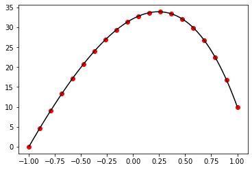
Exercise 11.6:
def f(x):
    return -50.0 * np.exp(x)

a = -1.0
b = 1.0
alpha = 00.0
beta = 10.0
n = 20

x_numerical, T_numerical = finite_element_method(f, a, b, n, alpha, beta)

x_analytical = np.linspace(a, b, 100)
T_analytical = -50.0 * np.exp(x_analytical) + 63.76 * x_analytical + 82.15

fig, ax = plt.subplots()
ax.scatter(x_numerical, T_numerical, color="red")
ax.plot(x_analytical, T_analytical, color="black")
plt.show()